Shell Equation Properties and Models
In this section we list all “material-region” specific models and properties associated with GOMA’s extensive shell equation capability. Currently we have specialized shell equations for Reynolds lubrication flow (lubp), open Reynolds film flow (shell_film_H), energy (shell_energy, convection and diffusion, coupled with lubrication), thin porous media (closed cell and open cell), melting and phase change and more. While many of these cards are actual material properties, most are geometry and kinematic related. The most appropriate place for these cards are region/ material files because they are actually boundary conditions and related parameters which arise from the reduction of order (integration through the thin film). For more information, please see the shell-equation tutorial (GT-036).
Upper Height Function Constants
Upper Height Function Constants = {model_name} <floatlist>
Description / Usage
This card takes the specification of the upper-height function for the confined channel lubrication capability, or the lub_p equation. This function specifies the height of the channel versus distance and time. Currently three models for {model_name} are permissible:
CONSTANT_SPEED |
This model invokes a squeeze/separation velocity uniformly across the entire material region, viz. the two walls are brought together/apart at a constant rate. This option requires two floating point values
|
ROLL_ON |
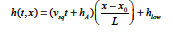
This model invokes a squeeze/separation velocity in a hinging-motion along one boundary. The model is best explained with the figure in the technical discussion section. The equation for the gap h as a function of time and the input parameters (floats) is as follows:
|
ROLL |
This model is used for a roll coating geometry. This option requires 8 floats:
|
FLAT_GRAD_FLAT |
This model used two arctan functions to mimic a flat region, then a region of constant slope, then another flat region. The transitions between the two regions are curved by the arctan function. This currently on works for changes in the x direction. This option requires five floating point values
|
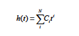
POLY_TIME |
This time applies a time-dependent lubrication height in the form of a polynomial. It can take as many arguments as GOMA can handle, and the resulting height function is
|
JOURNAL |
This model simulates a journal bearing. It is intended to be run on a cylindrical shell mesh aligned along the z axis and centered at (0,0). It could be extended to be more flexible, but this is all it is currently capable of. The height is defined by h(θ ) = C(1+ε cos(0)) Where C is the mean lubrication height and is the eccentricity of the two cylinders, with the smallest gap in the –y direction.
|
EXTERNAL_FIELD |
Not recognized. Oddly, this model is invoked with the extra optional float on the CONSTANT_SPEED option. |
External Field = HEIGHT Q1 name.exoII (see this card)
Examples
Following is a sample card:
Upper Height Function Constants = CONSTANT_SPEED {v_sq = -0.001} {h_i=0.001}
This results in an upper wall speed of 0.001 in a direction which reduces the gap, which is initial 0.001.
Technical Discussion
The material function model ROLL_ON prescribes the squeezing/separation motion of two non-parallel flate plates about a hinge point, as shown in the figure below.
Lower Height Function Constants
Lower Height Function Constants = {model_name} <floatlist>
Description / Usage
This card takes the specification of the lower-height function for the confined channel lubrication capability, or the lub_p equation. This function specifies the height of the channel versus distance and time. Currently three models for {model_name} are permissible:
CONSTANT_SPEED |
This model invokes a squeeze/separation velocity uniformly across the entire material region, viz. the two walls are brought together/apart at a constant rate. This option requires two floating point values
|
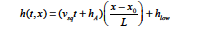
ROLL_ON |
This model invokes a squeeze/separation velocity in a hinging-motion along one boundary. The model is best explained with the figure in the technical discussion section. The equation for the gap h as a function of time and the input parameters (floats) is as follows:
|
ROLL |
This model is used for a roll coating geometry. This option requires 8 floats:
|
TABLE <integer1> <character_string1> {LINEAR | BILINEAR} [integer2] [FILE = filenm] |
Please see discussion at the beginning of the material properties Chapter 5 for input description and options. Most likely character_string1 will be LOWER_DISTANCE This option is good for inputing table geometry versus distance. Specifically, an arbitrary lower height function model is input as a function of the x-direction coordinate of the Lower Velocity Function model. This option in turn requires the use of SLIDER_POLY_TIME lower velocity function model. See example below. |
Examples
Following is a sample card:
Lower Height Function Constants = CONSTANT_SPEED {v_sq = -0.001} {h_i=0.001}
This results in an lower wall speed of 0.001 in a direction which reduces the gap, which is initial 0.001.
In another example:
Lower Height Function Constants = TABLE 2 LOWER_DISTANCE 0 LINEAR FILE=shell.dat
where shell.dat is a table with 2 columns, the first the position, the second the height.
Technical Discussion
The material function model ROLL_ON prescribes the squeezing/separation motion of two non-parallel flate plates about a hinge point, as shown in the figure below.
Upper Velocity Function Constants
Upper Velocity Function Constants = {model_name} <floatlist>
Description / Usage
This card takes the specification of the upper-wall velocity function for the confined channel lubrication capability, or the lub_p equation. This function specifies the velocity of the upper channel wall as a function of time. Currently two models for {model_name} are permissible:
CONSTANT |
This model invokes a squeeze/separation velocity uniformly across the entire material region, viz. the two walls are brought together/apart at a constant rate. This option requires two floating point values
|
ROLL |
This model invokes a wall velocity which corresponds to a rolling-motion. This model takes nine constants ???? :
|
TANGENTIAL_ROTATE |
his model allows a velocity that is always tangential to a shell surface, not necessarily aligned along the coordinate directions. It requires three specifications. First, a vector (v) that is always non-colinear to the normal vector of the shell must be specified. This is used to make unique tangent vectors. The last two specifications are the two tangential components to the velocity. The first velocity is applied in the direction of t1 = v×n. The second velocity is then applied in the t = t ×n direction.
|
CIRCLE_MELT |
Model which allows a converging or diverging height that is like a circle. Also works for melting.
|
Examples
Following is a sample card:
Upper Velocity Function Constants = CONSTANT {v_x= -0.001} {vy=0.00} {vz=0}
This card results in an upper wall speed of -0.001 in the x-direction which is tangential to the substrate, thus generating a Couette component to the flow field.
Technical Discussion
For non-curved shell meshes, most of the time they are oriented with the x-, y-, or zplane. This card is aimed at applying a tangential motion to that plane, and so one of the three components is usually zero.
Lower Velocity Function Constants
Lower Velocity Function Constants = {model_name} <floatlist>
Description / Usage
This card takes the specification of the Lower-wall velocity function for the confined channel lubrication capability, or the lub_p equation. This function specifies the velocity of the Lower channel wall as a function of time. Currently two models for {model_name} are permissible:
CONSTANT |
This model invokes a squeeze/separation velocity uniformly across the entire material region, viz. the two walls are brought together/apart at a constant rate. This option requires two floating point values
|
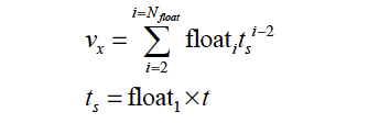
SLIDER_POLY_TIME |
This model implements a spatially-uniform velocity in the x-direction that is specified as a polynomial in time. The value of time may be scaled by a given scaling factor and the polynomial may have an unlimited number of terms.
|
ROLL |
This model invokes a wall velocity which corresponds to a rolling-motion. This model takes nine constants ???? :
|
TANGENTIAL_ROTATE |
This model allows a unique specification of tangential motion in a lubrication shell element. Previous implementations allowed specification only in terms of coordinate direction, but this option can be used to rotate a cylinder. Five floats are required
|
Examples
Following is a sample card:
Lower Velocity Function Constants = CONSTANT {v_x= -0.001} {vy=0.00} {vz=0}
This card results in an Lower wall speed of -0.001 in the x-direction which is tangential to the substrate, thus generating a Couette component to the flow field.
Technical Discussion
For non-curved shell meshes, most of the time they are oriented with the x-, y-, or zplane. This card is aimed at applying a tangential motion to that plane, and so one of the three components is usually zero.
Upper Contact Angle
Upper Contact Angle = {model_name} <floatlist>
Description / Usage
This card sets contact angle of the liquid phase on the upper-wall for the two-phase capability in the lub_p equation (viz. when using the level-set equation to model the motion of a meniscus in a thin gap, where the in-plan curvature is neglected. Currently one model {model_name} is permissible:
CONSTANT |
This model is used to set a constant contact able of the the free surface at the upper wall. Contact angle of less than 90 degrees is considered as nonwetting with respect to the heavier level-set phase. Only one floating point value is required.
|
Examples
Following is a sample card:
Upper Contact Angle = CONSTANT 180.
This card results in an upper wall contact able to 180 degrees, which is perfectly wetting. If the lower wall is given the same angle, then the capillary pressure jump will go as 2/h, where h is the gap.
Lower Contact Angle
Lower Contact Angle = {model_name} <floatlist>
Description / Usage
This card sets contact angle of the liquid phase on the lower-wall for the two-phase capability in the lub_p equation (viz. when using the level-set equation to model the motion of a meniscus in a thin gap, where the in-plan curvature is neglected. Currently one model {model_name} is permissible:
CONSTANT |
This model is used to set a constant contact able of the the free surface at the lower wall. Contact angle of less than 90 degrees is considered as nonwetting with respect to the heavier level-set phase. Only one floating point value is required.
|
Examples
Following is a sample card:
Lower Contact Angle = CONSTANT 180.
This card results in an lower wall contact able to 180 degrees, which is perfectly wetting. If the lower wall is given the same angle, then the capillary pressure jump will go as 2/h, where h is the gap.
Lubrication Fluid Source
Lubrication Fluid Source = {model_name} <floatlist>
Description / Usage
This card sets a fluid mass source term in the lub_p equation. Can be used to specify inflow mass fluxes over the entire portion of the lubrication gap in which the lub_p equation is active (over the shell material). This flux might be the result of an injection of fluid, or even melting. Currently two models {model_name} are permissible:
CONSTANT |
This model is used to set a constant fluid source in units of velocity. Only one floating point value is required.
|
MELT |
This model is used to set fluid source in units of Velocity which results from an analytical model of lubricated melt bearing flow due to Stiffler (1959). Three floating point values are required.
|
Lubrication Momentum Source
Lubrication Momentum Source = {model_name} <floatlist>
Description / Usage
This card sets a fluid “body force per unit volume” source term in the lub_p equation. This capability can be used to specify a force field over the entire shell area (over the shell material).. Currently two models {model_name} are permissible:
CONSTANT |
THIS MODEL NOT IMPLEMENTED AS OF 11/11/2010. This model is used to set a constant fluid momentum source in units of force per unit volume. Only one floating point value is required.
|
JXB |
This model is used to set fluid momentum source in units of force per unit volume which comes from externally supplied current density J field and magnetic B fields. These fields are suppled with the external field capability in Goma in a component wise fashion. Please consult the technical discussion below.
|
Technical Discussion
The two vector fields J, the current flux, and B, the magnetic induction, must be supplied to Goma in order to activate this option. At present, these fields must be supplied with the External Field cards, which provide the specific names of nodal variable fields in the EXODUS II files from which the fields are read. The three components of the J field must be called JX_REAL, JY_REAL, and JZ_REAL. Likewise the B field components must be called BX_REAL, BY_REAL, and BZ_REAL. These names are the default names coming from the electromagnetics code like Alegra. Because of the different coordinate convention when using cylindrical components, the fields have been made compatible with those arising from TORO II. It is the interface with TORO that also makes the Lorentz scaling (lsf) necessary so that the fixed set of units in TORO (MKS) can be adjusted to the user-selected units in Goma.
References
No References.
Turbulent Lubrication Mode
Turbulent Lubrication Model = {model_name}
Description / Usage
This card activates a turbulent model for viscosity in the lub_p equation. Currently one model {model_name} is permissible:
PRANDTL_MIXING |
This model is used to determine the pre-multiplier on the molecular viscosity in the Reynolds lubrication equation. For confined, laminar flow, this multiplier is 12. For turbulent flow it is taken as K(Re), where Re is the local Reynolds number. Specifically, invoking a analytical approximation for K from Hirs (1973), we set k0 according to the: Reynolds number Re= :ρh U μ For 0 < Re < 2000 K0=12 (Laminar case), Else 2000 < Re < 100000 K0 = 0.05Re 3/4 Here the wall velocity is used to compute The Reynolds number, as this turbulence model is specific to turbulent Couette flow. |
Technical Discussion
Several other models can be implemented in this instance. We chose this simple model which derives from Prandtl mixing length theory.
References
G.G. Hirs, “Bulk flow theory for turbulence in lubricant films”, Trans. ASME, ser. F, 95, pp 137-146, 1973.
Shell Energy Source QCONV
Shell Energy Source QCONV = {model_name} <float_list>
Description / Usage
This card activates a heat source (or sink, as it were) in the shell_energy equation. The functional form of this source/sink is a lumped heat-transfer coefficient model, hence the QCONV in its name (see BC = QCONV card in main user manual). Currently two models {model_name} are permissible:
CONSTANT |
This model invokes a simple constant heat-transfer coefficient and reference temperature, viz. q = H(T − Tref ). Commensurately there are two floats required: <float1> - Heat transfer coefficient in units of Energy/time/L2/deg T E.g. W/m2-K in MKS units. <float2> - Reference temperature. |
MELT_TURB |
This model also invokes a lumped parameter model, but the heat-transfer coefficient depends on the flow strength (Reynolds number), viz. q = H(T − Tref ). Three floats are required: <float1> - Thermal conductivity in units of Energy time/L/deg (e.g. W/m/k). <float2> - Reference temperature. <float3> - Latent heat of melting (Energy/M, e.g. J/Kg). This quantity is required due to the cross use of this in the shell_deltah equation (viz. EQ = shell_deltah). |
Examples
Following is a sample card:
Shell Energy Source QCONV = MELT_TURB {thermal_conductivity} {Tref} {latent_heat}
Technical Discussion
The MELT_TURB model warrants further discussion. The functional form of the heat transfer coefficient H is
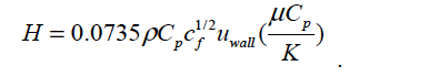
Here cf is the coefficient of friction, which for now is taken as 8./Re.
Shell Energy Source Sliding Contact
Shell Energy Source Sliding_Contact = {model_name} <float_list>
Description / Usage
This card activates a heat source (or sink, as it were) in the shell_energy equation. The functional form of this source/sink is a sliding contact model derived in the frame-of-reference of the slider on a stationary surface, so that the surface is moving in the simulation. In this case, the conditions for the flux vary from the leading edge to the trailing edge of the slider as a thermal boundary layer builds up. Think of this as a hot slider moving over a cold stationary wall, so that the flux at the leading edge of the slider into the cold wall will be larger, due to a steeper thermal boundary layer. Clearly the contact time will play a role. Currently two models {model_name} are permissible:
LOCAL_CONTACT |
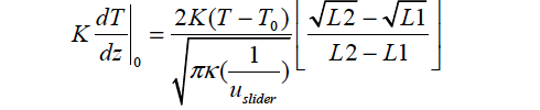
This model invokes the following functional form: Commensurately there are seven floats required:
|
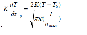
AVERAGE_CONTACT |
This model invokes the following functional form: Commensurately there are seven floats required:
|
Examples
Following is a sample card:
Shell Energy Source Sliding_Contact = LOCAL_CONTACT {L= 2.5} {t_r=20} {t_cond_cu_cgs} {density_cu_cgs} {heat_capacity_cu_cgs} {delta_L = 0.1} {leading_edge_coordx = 2.5}
Technical Discussion
Technical Discussion This boundary condition was derived using the analytical solution for heat conduction into an infinite slab, as derived by Carslaw and Jaeger. The modification here is that the temperature source accommodates a motion relative to the substrate, which is what leads to the need to segment the slider into bins over which a local heat flux solution is derived.
NOTE: If this card is used and there is no upper-wall or lower wall sliding motion, and error is thrown.
Shell Energy Source Viscous Dissipation
Shell Energy Source Viscous Dissipation = {model_name} <float_list>
Description / Usage
This card activates a heat source (or sink, as it were) in the shell_energy equation resulting from viscous dissipation due to shear combined Couette and pressure-driven flow in the Reynolds lubrication equation (lubp equation).
LUBRICATION |
This model invokes a viscous dissipation model simplified for the lubrication approximation.
|
LUBRICATION_FRICTION |
This model invokes the same viscous dissipation source term as in the LUBRICATION model, but adds on an additional linear friction model of the form μ*Pload vslider. Commensurately there are seven floats required:
|
Examples
Following is a sample card:
Shell Energy Source Viscous Dissipation= LUBRICATION_FRICTION {load=5e8} {coeff=0.9}
References
No References.
Shell Energy Source External
Shell Energy Source Viscous External = {model_name} <float_list>
Description / Usage
This card activates a heat source (or sink, as it were) in the shell_energy equation which corresponds to a user-supplied or constant value. Two models are available.
CONSTANT |
This model invokes a constant heat source term (heat sink if negative) in units of energy per area per time.
|
JOULE |
This model invokes a constant energy source which is determined by an external current density field of the form Qjoule = hξ J ⋅ J. Here J is the current density, h is the gap, and is the electrical resistivity, or the inverse conductivity. Both h and ξ are determined from other models in the material file. J is brought in as an external field variable from another exodusII file (see discussion below).
|
JOULE_LS |
This model differs from JOULE only in that the electrical conductivity is pulled out and must be specified with a LEVEL_SET model. This model is not well tested (PRS 12/14/2012)
|
Technical Discussion
To bring in an external field of the appropriate form, see the main Goma user’s manual and refer to the External Field card. As an example, you might consider solving a simple electrostatic problem using the EQ = V (voltage) equation and output the magnitude of the current density vector. In Goma, this is done with the post processing
Electric Field Magnitude = yes
Card. This card outputs this J-magnitude as the exodusII variable EE. You then bring it in as follows in the input script:
External Field = EE Q1 current_dens_out.exoII
With the JOULE model, this field is used to compute the Joule heating term.
References
No References.
FSI Deformation Model
FSI Deformation Model = {model_name}
Description / Usage
This card specifies the type of interaction the lubrication shell elements will have with any surrounding continuum element friends. When not coupling the lubrication equations to a continuum element, this card should be set to the default value, FSI_SHELL_ONLY. All models are described below:
FSI_MESH_BOTH This model should be used when both the shell and neighboring continuum elements use deformable meshes and the user wishes to full couple these behaviors. This model is not currently implemented and should not be used.
FSI_MESH_CONTINUUM In this model, the neighboring continuum elements use mesh equations, but the lubrication shell does not. This model features a two-way coupling, where the lubrication pressure can deform the neighboring solid (through the appropriate boundary condition) and deformations to the mesh in turn affect the height of the lubrication gap. This is equivalent to the old “toggle = 1”.
FSI_MESH_SHELL This model accounts for mesh equations present in the lubrication shell, but not in the adjoining continuum elements. This model is not currently implemented and should not be used.
FSI_SHELL_ONLY This model can be thought of as the default behavior, where there is no coupling between the lubrication shell elements and any neighboring continuum elements. This should also be used if only shells are present.
FSI_MESH_UNDEF This model is similar to FSI_MESH_CONTINUUM, but the normal vectors in the shell are calculated using the original undeformed configuration, rather than the current deformed state. Implementation of this model is currently in progress and needs to be fully tested.
FSI_MESH_ONEWAY This model is similar to FSI_MESH_CONTINUUM, but only utilizes a one way coupling. Deformations in the neighboring continuum element do not affect the lubrication height, but do affect the calculated normal vectors. This is equivalent to the old “toggle = 0”.
Examples
Technical Discussion
References
No References.
Film Evaporation Model
Film Evaporation Model = {model_name} <floatlist>
Description / Usage
This card takes the specification of the evaporation rate for the film-flow equation capability, specifically the shell_filmp equation. This function specifies the rate of evaporation in the unit of length per time. Currently two models for {model_name} are permissible:
CONSTANT |
This model specifies a constant evaporation rate. This option requires one floating point values
|
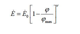
CONC_POWER |
This model specifies evaporation rate function of particles volume fraction and the input parameters (floats). This model is proposed by Schwartz et al (2001). The functional form is:
|
Examples
Following is a sample card:
Film Evaporation Model = CONC_POWER 1.0e-3 0.5 0.64
This results in film evaporation with the pure liquid evaporation rate of 1.0e-3, exponent of 0.5, and maximum packing volume fraction of 0.64.
References
Leonard W. Schwartz, R. Valery Roy, Richard R. Eley, and Stanislaw Petrash, “Dewetting Patterns in a Drying Liquid Film”, Journal of Colloid and Interface Science 234, 363–374 (2001)
Disjoining Pressure Model
Disjoining Pressure Model = {model_name} <floatlist>
Description / Usage
This card takes the specification of the disjoining pressure model for the film-flow equation capability, specifically the shell_filmh equation. This function specifies the disjoining pressure in the unit of force per area. Currently four models for {model_name} are permissible:
CONSTANT |
This model specifies a constant disjoining pressure. This option requires one floating point values
|
ONE_TERM This model specifies disjoining pressure and the input parameters (floats). This model only employs the repulsion part of the van der Waals force. The functional form is:
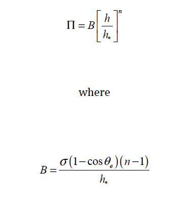
<float1> is the equilibrium liquid-solid contact angle θe
<float2> is exponent n and it should satisfy n >1
<float3> is the precursor film thickness h*
TWO_TERM This model specifies disjoining pressure and the input parameters (floats). Here, the model only employs both repulsion and attraction part of the van der Waals force. The functional form is:
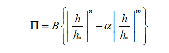
where
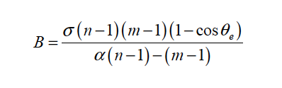
<float1> is the equilibrium liquid-solid contact angle 0e
<float2> is exponent n corresponding to the repulsive part of the van der Waals force. It should satisfy n >1
<float3> is exponent m corresponding to the attractive part of the van der Waals force. It should satisfy m > n since the attractive part acts in longer range than the repulsive one.
<float4> is the precursor film thickness h
<float5> is the parameter a describing relative importance of the attractive part to the repulsive part. Typically, a is chosen to be 0 <α <1 in order to achieve more numerical stability.
TWO_TERM_EXT_CA This model is identical with TWO_TERM except that it uses contact angle from an external field identifies as THETA.
Examples
Following is a sample card:
Disjoining Pressure Model = TWO_TERM 120.3 2 1.0e-4 0.1
This results in disjoining pressure with contact angle of 120, repulsive exponent of 3, attractive repulsion of 2, precursor film thickness of 1.0e-4, and relative importance of attractive part of 0.1.
Technical Discussion
A thorough discussion of disjoining pressure can be found in Teletzke et al (1987). The premultiplying constant is related to contact angle and surface tension by balancing capillary and disjoining force where the wetting line meets the precursor film. See Schwartz (1998) for further detail.
References
Leonard W. Schwartz, R. Valery Roy, Richard R. Eley, and Stanislaw Petrash, “Dewetting Patterns in a Drying Liquid Film”, Journal of Colloid and Interface Science 234, 363–374 (2001)
Teletzke, G. F., Davis, H. T., and Scriven, L. E., “How liquids spread on solids”, Chem. Eng. Comm., 55, pp 41-81 (1987).
Diffusion Coefficient Model
Diffusion Coefficient Model = {model_name} <floatlist>
Description / Usage
This card takes the specification of the diffusion coefficient model for the conservation of particles inside film-flow capability, i.e. equation describing shell_partc. Currently two models for {model_name} are permissible:
CONSTANT |
This model specifies a constant diffusion coefficient. This option requires one floating point values
|
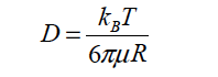
STOKES_EINSTEIN |
This model specifies diffusion coefficient that depends on particles radius and the film viscosity. The functional form is:
|
Examples
Following is a sample card:
Diffusion Coefficient Model = STOKES_EINSTEIN 1.3807e-16 298 1.0e-6
This results in diffusion coefficient calculated with Stokes Einstein model with Bolztmann constant of 1.3807e-16 in CGS units, 298 K temperature, and 1.0e-6 cm radius particles.
Technical Discussion
Viscosity dependence of diffusion coefficient can be exploited to relate particles concentration (or volume fraction in this case) to diffusion coefficient by employing SUSPENSION viscosity model in the material file. See SUSPENSION viscosity model for further detail
Porous Shell Radius
Porous Shell Closed Radius = {model_name} <floatlist>
Description / Usage
This card specifies the radius of the pores used in porous_shell_closed and porous_shell_open equations. Currently two models for {model_name} are permissible:
CONSTANT |
This model applies a constant pore radius for the entire model. It requires a single floating point value.
|
EXTERNAL_FIELD |
This model reads in an array of values for the radius from an initial exodus file. This allows for spatial variations in the parameter value. |
References
No References.
Porous Shell Height
Porous Shell Height = {model_name} <floatlist>
Description / Usage
This card specifies height of the pores used in porous_shell_closed and porous_shell_open equations. Currently two models for {model_name} are permissible:
CONSTANT |
This model applies a constant pore height for the entire model. It requires a single floating point value.
|
EXTERNAL_FIELD |
This model reads in an array of values for the height from an initial exodus file. This allows for spatial variations in the parameter value. |
References
No References.
Porous Shell Closed Porosity
Porous Shell Closed Porosity = {model_name} <floatlist>
Description / Usage
This card specifies the porosity used in porous_shell_closed equations. Currently two models for {model_name} are permissible:
CONSTANT |
This model applies a constant porosity for the entire model. It requires a single floating point value.
|
EXTERNAL_FIELD |
FIELDThis model reads in an array of values for the porosity from an initial exodus file. This allows for spatial variations in the parameter value.
The ExodusII field variable name should be “SH_SAT_CL_POROSITY”, viz. |
External Field = SH_SAT_CLOSED_POROSITY Q1 name.exoII (see this card)
References
No References.
Porous Shell Closed Gas Pressure
Porous Shell Closed Gas Pressure = {model_name} <floatlist>
Description / Usage
This card specifies the gas pressure used in porous_shell_closed equations. Currently one model for {model_name} are permissible:
CONSTANT |
This model applies a constant gas pressure for the entire model. It requires a single floating point value.
|
References
No References.
Porous Shell Atmospheric Pressure
Porous Shell Atmospheric Pressure = {model_name} <floatlist>
Description / Usage
This card is used to set the atmospheric pressure level in a open-cell shell porous equation (for partially saturated flow). As of 11/27/2012 this card is NOT used.
Examples
No Examples.
References
No References.
Porous Shell Reference Pressure
Porous Shell Atmospheric Pressure = {model_name} <floatlist>
Description / Usage
This card is used to set the reference pressure level in a open-cell shell porous equation (for partially saturated flow). This pressure is used to shift the saturation-capillary pressure curve appropriately. As of 11/27/2012 this card is NOT used as all saturation curve information is handled in the main porous flow property input framework, even for shell formulations.
Examples
No Examples.
References
No References.
Porous Shell Cross Permeability
Porous Shell Cross Permeability = {model_name} <floatlist>
Description / Usage
This card is used to set the permeability in the thin direction of a shell porous region. The property is used for the porous_sat_open equation. The in-shell (in-plane for a flat shell) permeabilities are set on the Permeability card. Please consult the references for the equation form. The property can take on one of two models:
CONSTANT |
This model applies a constant cross-region permeability. It requires a single floating point input:
|
EXTERNAL_FIELD |
This model is used to read a finite element mesh field representing the cross-term permeability. Please consult tutorials listed below for proper usage. This model requires one float:
The ExodusII field variable name should be “CROSS_PERM”, viz. |
Examples
No Examples.
References
Roberts and P. R. Schunk 2012. in preparation.
Randy Schunk 2011. GT-038 “Pixel-to-Mesh-Map Tool Tutorial for GOMA”. Memo to distribution.
Porous Shell Gas Diffusivity
Porous Shell Gas Diffusivity = {model_name} <floatlist>
Description / Usage
This card is used to set the gas diffusivity for the trapped gas in the porous_sat_closed equation. Basically, the gas trapped in closed pores during the imbibition process is allowed to diffuse into the liquid, and this property is a part of that model gas inventory equation R_SHELL_SAT_GASN. Only one model is available for this property:
CONSTANT |
This model applies a constant cross-region permeability. It requires a single floating point input:
|
EXTERNAL_FIELD |
This model applies a constant gas diffusivity. It requires a single floating point input:
|
Examples
Porous Shell Gas Diffusivity = CONSTANT 1.e-5
References
Roberts and P. R. Schunk 2012. in preparation.
Porous Shell Gas Temperature Constant
Porous Shell Gas Temperature Constant = {model_name} <floatlist>
Description / Usage
This card is used to set the temperature constant in Henry’s law for the trapped gas in the porous_sat_closed equation. Basically, the gas trapped in closed pores during the imbibition process is allowed to diffuse into the liquid, and this property is a part of that model for the dissolution constant of gas in pressurized liquid. It is only needed if the equation R_SHELL_SAT_GASN is used. Only one model is available for this property:
CONSTANT |
This model sets the Henry’s law temperature constant. It requires a single floating point input:
|
Examples
Porous Shell Gas Temperature Constant= CONSTANT 1.e10
References
Roberts and P. R. Schunk 2012. in preparation.
Porous Shell Henrys Law Constant
Porous Shell Henrys Law Constant = {model_name} <floatlist>
Description / Usage
This card is used to set the partitionconstant in Henry’s law for the trapped gas in the porous_sat_closed equation. Basically, the gas trapped in closed pores during the imbibition process is allowed to diffuse into the liquid, and this property is a part of that model for the dissolution constant of gas in pressurized liquid. It is only needed if the equation R_SHELL_SAT_GASN is used. Please consult the references for a detailed explanation. Only one model is available for this property:
CONSTANT |
This model sets the Henry’s law constant. It requires a single floating point input:
|
Examples
Porous Shell Gas Temperature Constant= CONSTANT 1.e10
References
Roberts and P. R. Schunk 2012. in preparation.